A little history

As technology advances so must problem-solving techniques. With global markets, complex electronic devices, ever larger engineering projects, it is not always possible to have closed-form solutions to the equations governing the dynamics of a given system. As a result, several numerical techniques have been developed to help understand the complexities of the systems being investigated. For example, the equations governing fluid dynamics systems are often systems of partial differential equations (PDEs) that cannot be solved “by hand.” Finite difference schemes are one way to numerically solve these systems. In mathematical finance, the high dimensional nature of markets makes a PDE approach very cumbersome. As such, there has been considerable research and development by academics and practitioners in the use of simulation techniques to value options and other derivatives, among other things, under a risk-neutral framework. These simulation techniques are often referred to as “the Monte Carlo method.”

The name “Monte Carlo” comes from the popular Monte Carlo casino in Monaco and was coined by physicists working on atomic weapons projects in the 1940s [N. Metropolis and S. Ulam. The monte carlo method Journal of the American Statistical Association, 44:335–341, 1949.]. The history of the Monte Carlo method is much older than its namesake. One of the first recorded simulation experiments dates back to the 1700s! This is Buffon’s Needle Problem to approximate \(\pi\) [G. Buffon. Essai d’arithmétique morale Histoire naturelle, générale er particulière, 4:46–123, 1777.]. However, given the nonexistent computing resources available in the 1700s, simulation techniques were not necessarily a practical problem solving method. As computing power has grown, the Monte Carlo method has become increasingly popular and has been demonstrated to be a reliable problem solving technique.

While the Monte Carlo method is an advanced problem solving technique and is widely used in a variety of disciplines (e.g., finance and particle physics to name just a few), it is usually only taught at the graduate level and only in certain disciplines. This is not without good reason — there is a considerable amount of probability theory, applied statistics, and knowledge of programming that is required in order to use the technique in an industrial setting. On the other hand, the Monte Carlo method is conceptually very easy to understand and as such it can be used as an educational tool from grade school to graduate school.

A motivational example

The Monte Carlo method has gained tremendous popularity in a variety of industries because of its noticeable amount of success in the estimation of solutions to high-dimensional problems.

One can understand the basic need for and principles underlying the Monte Carlo method through the following example: suppose on a sheet of paper we draw some shapes like that in Figure 1. Next, suppose we want to know the area covered by these shapes as a percentage of the area of the drawing region. How do we do this? There are likely many ways. The Monte Carlo method would estimate this area in a probabilistic manner.

Figure 1: A random drawing — we want to estimate the area of the shaded region as a percentage of the canvas on which it is drawn

Suppose now, that we have access to darts with very fine tips. Hanging the artwork on a wall and standing at a reasonable distance so that our aim would be worthless, we throw darts at the paper. After throwing a good many of them, we count the number of darts that landed inside the drawn region and divide it by the total darts thrown to give us an estimate for the area as a percentage of the area of the paper! This is, effectively, the Monte Carlo method.

On a computer, we can simulate this act of dart throwing. What this amounts to is 1) choosing points at random from a uniform distribution on some rectangle in the \(x\)-\(y\) plane that bounds the objects whose area is to be estimated, 2) counting the number of points that landed within the boundary of the objects, and 3) computing the ratio of the points that landed within the boundary of the objects to the total number of random points used. This gives an estimate for the area covered by the objects as a percentage of the bounding rectangle. The more random points used, the better the estimate. Figure 2 shows an example of this.

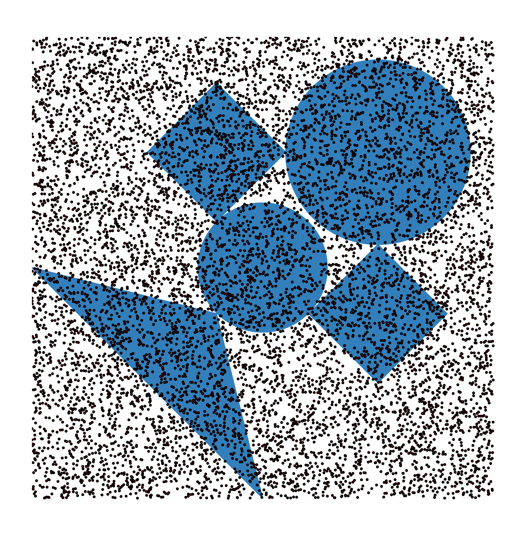
Figure 2: A Monte Carlo estimate for the area encompassed by the shaded region is 36.6% of the bounding rectangle — 3,660 of the 10,000 points used landed within the shaded region

In the example of Figure 2, the shapes were all distinct and hence one could compute the area using known formulas for area. However, when the regions become more complicated, analytical solutions are not always possible. Figures 3 and 4 show how we can use the Monte Carlo method even when the region begins to get more complicated.

Figure 3: A more complicated region for which direct methods to compute the area may not work very easily

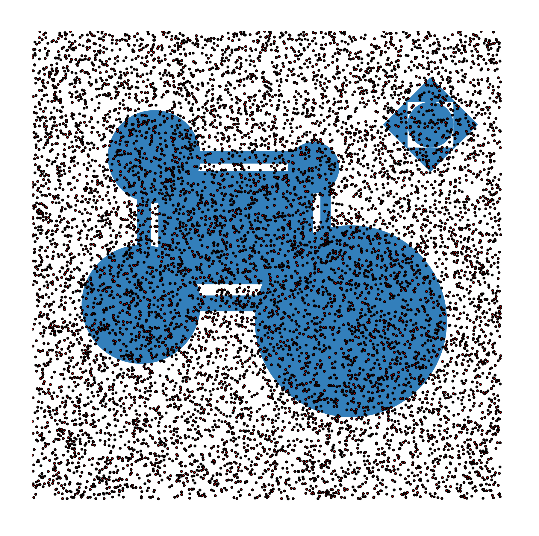
Figure 4: A Monte Carlo estimate for the area encompassed by the shaded region is 31.35% of the bounding rectangle — 3,135 of the 10,000 points used landed within the shaded region

This technique of “throwing darts” is known as the “Hit or Miss Monte Carlo method” [Reuven Y. Rubinstein. Simulation and the Monte Carlo Method John Wiley & Sons, New York, 1981.]. One can see that an immediate application of the Hit or Miss method is for numerical integration. Geometrically, integration is understood as “area under the curve”. Thus one way to estimate \(\displaystyle \int_{a}^{b} f(x)\ dx\) is to find values \(c\) and \(d\) such that \(c \leq f(x) \leq d\) for all \(x\in[a,b]\) and sample at random from a uniform distribution in the rectangle \([a,b] \times [c,d]\). If the random point \(p = (p_{x}, p_{y})\) gives \(f(p_{x}) \geq p_{y}\), then we record a hit. If the random point \(p = (p_{x}, p_{y})\) gives \(f(p_{x}) \leq p_{y}\) then we record a miss. Then if \(n_{h}\) is the number of hits and \(n\) is the number of random points used, we have $$\int_{a}^{b}f(x)\ dx \approx \frac{n_{h}}{n}(b-a)(d-c)$$ The results of Figures 2 and 4 were the ratio \(\frac{n_{h}}{n}\) — this represents the percent of the area of the rectangular bounding region that is covered by the shaded region or it can also be interpreted as the probability that a point chosen at random from the bounding region would land within the shaded region.

For further reading about the Monte Carlo method, see [Reuven Y. Rubinstein. Simulation and the Monte Carlo Method John Wiley & Sons, New York, 1981.]. Feel free to contact me if you are interested in learning about the technical details!