This post is part of the ppmmc series. Please make sure to have read the previous posts in the ppmmc series so that the context is understood.
In yesterday’s post we simulated the two games offered by Mr. Conner Tist. We found that while the second game gave us a 25% chance of winning compared to the \(\approx\)16.6% chance offered by the first game, we were actually losing more points playing the second game.
Now, these games were relatively simple. But simple things are a good starting point for us to learn a few things. So what we’ll do today is explain, intuitively, what the requirements are for something to considered a Markov chain.
A Very Introductory Introduction to Markov Chains — Part 4
If we consider our dice roll games (either one), we noticed that no matter what the history of dice rolls was the probability that we would go from win / lose / draw / reroll (if draw and reroll were possibility) from the previous roll to the next roll was always the same. Take for example, the first game — if the 2000th roll resulted in a draw, the probability that the 2001st roll will result in a draw is the same no matter which roll we considered. This is called the time-homogeneity property of Markov chains.
Argue, intuitively, that the second game is time-homonegenous.
Another property of Markov chains is that they must be memoryless. Memorylessness means just that — no matter what the history, the transition to the next state only depends on the current state. This property was not explicitly displayed in the two games because of their simplistic nature. Nevertheless, both of the dice games were memoryless. Suppose that we observed the following sequence of events in the first game: draw, draw, draw, draw. The probability that the fifth roll would result in a draw does not depend on the fact that the last four games resulted in a draw. But this is, in some sense, degenerate for our dice roll games. Thus, we will explore another game.
Markov Pinball
Consider five circles arranged in a pentagon. Suppose a ball is released from one of the circles. Which other circle it goes to is dictated as follows: The ball cannot go to a circle next to the circle it came from home nor can it go to itself. It can go to any other circle with equal probability.
Our state diagram would look like this. Does that make sense?
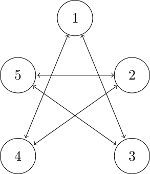
Now, we start using some standard notation to describe how we may transition from one state to the next. We write the probability that we transition from state \(i\) to state \(j\) given that we are in state \(i\) on time step \(k\) as \(p_{ij,k}\). In other words, the probability that going from state 1 to state 3 in time step 1 would be written as \(p_{13,1}\).
So, let’s get used to this notation. From the diagram above and the rule for transitions, we have, for examples, \(p_{13,1} = \frac{1}{2}\) and \(p_{15,1} = 0\)
Write out the \(p_{ij,k}\) for all the transitions given in the diagram above. Can you see that this is time-homogenous and memoryless? Are there any absorbing states?
A game of chance
Mr. Conner Tist is back with another game to offer. This time he claims that it is fair, i.e., that, on average, neither side has an advantage (the expected value is zero). Here is the game:
- Let’s say that the game always begins on state 1.
- Every time we land on 4, we lose three points.
- Every time we land on 2, 3, or 5, we gain a point.
- The game ends once we land back on 1.
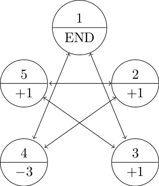
For example, since the game begins on state 1, we could have a game like this 1-3-5-2-5-2-4-1. The final tally would be two points in our favor (we three points for landing on 4 but gained five points for landing on 2s, 3s, and 5s). Another game could be 1-4-2-4-1 and we would lose a net of five points.
Is this game fair? Or are we being hustled again? Can you simulate this? Can you solve this “on paper”?
Don’t hesitate to get in touch if you have questions or would like more information about setting up a workshop or training in your school.
Pingback: Programming, Probability, and the Modern Mathematics Classroom — Part 13 | Math Misery?
Pingback: Programming, Probability, and the Modern Mathematics Classroom — Part 12 | Math Misery?