This post is part of the ppmmc series. Please make sure to have read the previous posts in the ppmmc series so that the context is understood.
In Thursday’s post (6/20) we observed that after 100 million game plays we had results that were very near the theoretical calculations. While the theoretical expected value for the game was zero, our simulations produced a slightly negative expected value over 100 million game plays. So we asked if this made sense. We ran another batch of 100 million plays and observed a negative expected value again, though very close to zero on a per game basis.
In this post, we want to begin to investigate the difference between our simulations and our theoretical calculations. For those with an introductory background in probability and statistics, or for instructors, you will know that we intend to discuss variance. If you’ve never heard this term before, then, for now, understand variance colloquially — something that is different. Unfortunately, the mathematical definition of variance doesn’t quite line up with the colloquial use of the word and this leads to all manners of confusion. The term “standard deviation” is more inline with the colloquial use of “variance”. In any case, just keep this in mind.
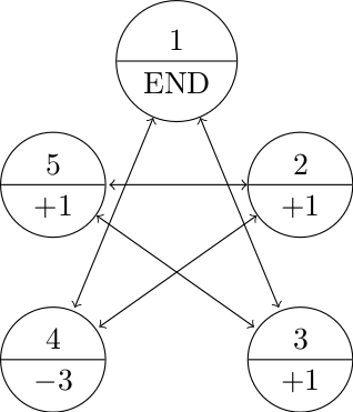
Recall the rules
- Let’s say that the game always begins on state 1.
- Every time we land on 4, we lose three points.
- Every time we land on 2, 3, or 5, we gain a point.
- The game ends once we land back on 1.
- The transition probabilities are all equal to \(\frac{1}{2}\) and the transitions are dictated by the state diagram below.
Understanding the Difference Between Simulated and Theoretical Results
One of the things we want to do is a get a handle on what is going on with our simulations. Our theoretical expected value was zero. Yet, two independent trials of 100 million simulations, produced negative results. How can we explain this?
For sake of sparing some computational resources, let’s see what happens if we run 20 batches of 5 million simulations per batch (this will give us a total of 100 million simulations). By now, we hope that our readers can modify the Python code appropriately. Below is one way of doing this. (Another way would be wrap the original game code into a function and then have another function run the simulations.
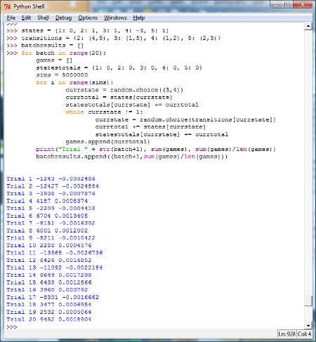
So, what do we notice? We can see that in the 20 batches of 5 million simulations per batch we had a mix of positive and negative returns on a per game basis. Is this good or bad?
In our case, since the expected value of the game was zero, it is a good thing that we have both positive and negative values.
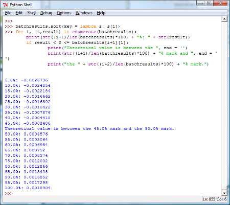
To get a handle on how good or bad this is, one thing we can do is sort the returns (this is why created the variable \(\mbox{batchresults}\)). Here is how to sort a list (this is new, so take some time out to experiment here!).
And now, let’s print our sorted list and see where the zero would be. The lowest value in the list would represent the bottom 5% of our data. This means that if the theoretical return of zero is less than the lowest value in the list, it would be in the bottom 5% of our data. The next lowest value in the list represents the 10% mark. The largest value in the list represents the 100% mark. The next highest value represents the 95% mark.
Just to be clear, this demarcation of percentiles doesn’t have to be the only way to do it. One could just as well say that the lowest value represents the bottom 2.5% while the largest value represents 97.5%. But we’ll get into the formalities of all this later.
Very loosely speaking, we want to decide a priori what our cutoff points are for what we would consider to be an “extreme” set of data points. For example, if we said that if the theoretical value were less than the lowest observed value or greater than the highest observed value, then we would suspect either our theoretical calculations or our simulations (or both). If that were not the case, then we would say with reasonable confidence that our simulated and our theoretical value corroborate each other.
One of the tricky things here is that if we cast too wide of a net, we’ll always have our simulated and theoretical values corroborating each other. On the other hand, if we are too narrow (say requiring that the theoretical value be between the 45% and 50% mark), we’ll find fault too often. Thus, in the experimental design, this decision has to be made carefully.
From the results, we can see that the simulated and theoretical values are indeed near each other, since the theoretical value is between the 45% and 50% mark. We can also see that of the twenty batches, nine of them had a negative simulated value and the other eleven were positive.
We’ll stop here for today, but as a simple exercise run this same experiment with 20 batches of 100 million simulations per batch.
Tomorrow we’ll continue with this.
Don’t hesitate to get in touch if you have questions or would like more information about setting up a workshop or training in your school.
Pingback: Programming, Probability, and the Modern Mathematics Classroom — Part 15 | Math Misery?