Genetic algorithms are a fun and sometimes almost magical problem solving tool. This write-up is a quick and dirty tutorial implementing a genetic algorithm to solve a particular geometry problem. I’ve often found it instructive to learn a new method, algorithm, technique on a problem I can already solve
First, let’s talk high-level. We’re going to first identify our problem mathematically. Then we’ll sample a region where we believe the solution should exist. And from there we’ll continue to refine our search. Now keep in mind that this problem will be easy to solve by hand, but our purpose here is to see how an evolutionary algorithm / method would find the solution.
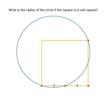
Here’s a pretty picture that I’ll explain and we’ll build off of!
The Problem
I have a unit square whose bottom left corner is anchored at \((0,0)\). A circle of unknown radius intersects my square at the following points: \((0,0), (0.5, 0), \mbox{ and }, (1,1)\). What is the radius of the circle? This was a puzzle from Ed Southall and @srcav blogged about it here.
It might help if we could draw this out.
This problem can be viewed in a number of different ways, but a coordinate geometry approach seems to be simplest, at least for me.
We want to know the circle’s radius given that we have a unit square and a number of intersection points.
This yields the following set of equations if \(h\) and \(k\) are the \(x\) and \(y\) coordinates of the center of the circle:
$$
\begin{eqnarray}
h^{2} + k^{2} & = & r^{2}\\
(0.5-h)^{2} + k^{2} & = & r^{2}\\
(1-h)^{2} + (1-k)^{2} & = & r^{2}
\end{eqnarray}
$$
Remember that the equation of a circle with center \((h,k)\) is $$(x-h)^{2} + (y-k)^{2} = r^{2}$$
We have three equations, three unknowns. The algebra is pretty straightforward to go through as the square terms drop out. But! You may say, “Damn it, Shah, it’s straightforward for you, it’s not easy for me!” However, you’ve got programming chops that are beyond mine. So let’s put that to work. There’s more than one way to skin a math problem!
An Approach
What we want are \(h\) and \(k\) from above and those values together should give the same value for \(r^{2}\) for each of the equations.
I’ll introduce the jargon of genetic algorithms as we need it. The first thing we want to do is create an initial “population”. Our population is a collection of points \((x,y)\) within some region where we believe the solution exists. To be conservative, let’s sample from a large enough space, say, something like \([-1,2]\times[-1,2]\). We know that we can definitely contain the circle in an area of 9 square units in that range.
How should we sample this region?
Uniform random sampling is a good place. And we can pick, say, 10,000 points at random.
What should we do we these points?
The first thing we want to do is assign a “fitness score” that tells us how good these points are. In this case, I want to see the largest absolute difference in \(r^{2}\) from all pairwise comparisons of the three equations. The larger the difference, the worse the fit. The closer the absolute difference is to zero, the better the fit. Here’s python code.
def opt(h,k):
    f1 = h**2 + k**2
    f2 = (0.5-h)**2 + k**2
    f3 = (1-h)**2 + (1-k)**2
    return max(abs(f1-f2), abs(f2-f3), abs(f1-f3)),((f1 + f2 + f3)/3)**0.5
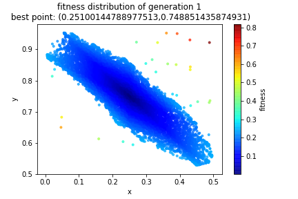
So, if I create an initial population of 10,000 random points in \([-1,2]\times[-1,2]\) and apply a fitness score to each of those points, I now have the following visualization of our sample space. Notice that the bluer the region, the better the fit.
Great, now what?
Ok! That was just an initial set up. Now the genetic part is going to come in. Each “individual” in the population is really a coordinate \((x,y)\). We can think of those dimensions as the “genetic code” for each individual. So, sticking with the analogy of evolutionary theory, we want to have a sort of “survival of the fittest” take place. That is, only the strong get to reproduce. Everyone else dies and their genetics do not get to passed on.
There are a lot of ways to do this and you can, for the most part, make up your own methodology, though there are some generally accepted principles and standards.
What we now have to do with this initial population is to pick two individuals and have them “mate”!
How do mathematical objects “mate”?
Glad you asked! There are a lot of ways to do this mating and, in general, the term is called “crossover” whereby the two selected individuals create some “offspring” which is composed of the two “parents” genetic code. Here is one example of a crossover in action.
Suppose we have an individual A with “DNA” \((0.3, 0.8)\) and another individual, B, with DNA \(0.1, 0.5\). We could produce offspring M as \((0.1, 0.8)\) and offspring N as \((0.3, 0.5)\). Notice that we just swapped the \(x\) and \(y\) coordinates!
Another way is “alpha-averaging”. Pick a real number \(\alpha \in (0,1)\) and produce offspring as the weighted average of the parents. Something like \(M = \alpha A + (1-\alpha) B\) and \(N = (1-\alpha) A + \alpha B\).
def arithmetic_crossover(pair,optfunc):
    alpha = random.random()
    offspring1 = [pair.iloc[0]['x']*alpha + pair.iloc[1]['x']*(1-alpha),pair.iloc[0]['y']*alpha + pair.iloc[1]['y']*(1-alpha)]
    offspring2 = [pair.iloc[0]['x']*(1-alpha) + pair.iloc[1]['x']*(alpha),pair.iloc[0]['y']*(1-alpha) + pair.iloc[1]['y']*(alpha)]
    score1 = optfunc(offspring1[0],offspring1[1])
    score2 = optfunc(offspring2[0],offspring2[1])
    df1 = [offspring1[0],offspring1[1],score1[0],score1[1]]
    df2 = [offspring2[0],offspring2[1],score2[0],score2[1]]
    return [df1,df2]
Who gets to mate?
It’s survival of the fittest! That’s why we computed a fitness score! There are several ways to decide on who gets to mate. Our goal is to pass on good individuals’ genes (in our case low fitness scores) to the next generation of offspring. This type of method is called “elitism”. You can choose how elitist you want to be. I chose to have the next population drawn from the top 1% of individuals per their fitness scores.
But there’s a catch! In this world of genetic reproduction, there is the possibility of a “mutation”. Think of mutation as a hedge against getting stuck in a local extremum when we are trying to optimize a function.
You might have caught on that there is a bit of ad-hocness to some of these parameters. How often should be mutate? It’s up to you! The higher the mutation rate, the closer the genetic algorithm is to a pure random search.
For this problem, I chose to reproduce from the top 1% of the population with 99% probability. With 1% probability I chose to draw a random individual from the bounding box of the current elite population (I could have chosen a wider range and doing so would be more inline with the hedge against getting stuck in local extrema).
Here’s code for how the next generation is created.
def next_pop(curr_pop, optfunc):
    n = curr_pop.shape[0]
    upperp = numpy.percentile(curr_pop['fitness'],1)
    q = curr_pop.query('fitness < {z}'.format(z = upperp))
    mins = q.min()
    maxs = q.max()
    pop = q.values.tolist()
    sz = len(pop)
    while len(pop) < n:
        if random.random() < .99:
            mates = q.sample(2)
            mates.reset_index(inplace = True,drop = True)
            offsprings = arithmetic_crossover(mates,optfunc)
            pop.append(offsprings[0])
            pop.append(offsprings[1])
        else:
            x = random.random()*(maxs['x']-mins['x']) + mins['x']
            y = random.random()*(maxs['y']-mins['y']) + mins['y']
            score = optfunc(x,y)
            fitness = score[0]
            average_radius = score[1]
            pop.append([x,y,fitness,average_radius])
    return pandas.DataFrame(pop,columns = ['x','y','fitness','average_radius']), len(pop)-sz
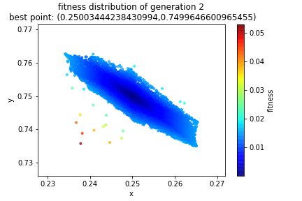
And that’s it! Now we just rinse and repeat! Here’s how the solution evolved. If you solved the equations by hand you should have gotten a center of \((0.25, 0.75)\) resulting in a radius of \(\frac{\sqrt{10}}{4}\). Notice in the title of the graphs, the best point found in each generation. I put the graph of the initial population in here for the third time in this post so that you can see how the initial random sample evolves.
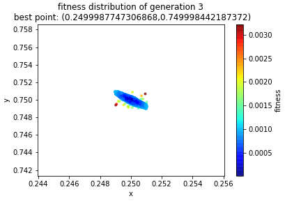
At this point we can feel that we have a fairly accurate solution. But when we stop is up to us! Often we will have an error tolerance set up to act as a stopping time. Other times, we may measure how much the solution has changed from one generation to the next to determine if there is still further room for improvement or if we’ve reached convergence.
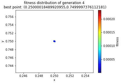
By the fourth generation we are pretty well locked into a small region and indeed we see to have convergence.
One piece of criticism!
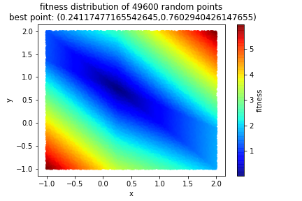
It can feel like we are cheating because we keep trying “random” numbers and we’re just getting lucky. This is not so! One of the things I track is how many unique points I try over all generations. I then want to do a pure random search on my initial [larger, low-informed] search space. If I obtain comparable results [you can define your own tolerance here] with the genetic algorithm, then I probably can just get away with pure random sampling. It turns out that, at least for this problem, our genetic algorithm is quite superior. In each generation I had a population of 10000 and in the aggregate over the five generations, I generated 49600 unique points (elitism kept about 100 per generation). Here’s what a pure random search with 49600 points produced.
As you can see, while we are in the ballpark with a purely random search, the genetic algorithm with just as many points produced a far more accurate number. And remember we wanted to find the radius of the circle. Since we have the center, it’s a matter of picking one of the points on the circle (\((0,0)\) as an easy example) and computing the distance. That’s our radius!
To Sum Up
If you want to continue to learn, DuckDuckGo is your friend, but now you have a bunch of terms (crossover, mutation, population, elitism) and a sample problem to work off of! Remember that the crossover functionality can be highly varied. We were working in a continuous framework. When we have to work in a discrete problem or a permutation problem, crossover works differently.
See if you can write your own genetic algorithm to maximize \(\sin(2\pi x) + \sin(2\pi y)\) on \([0,1]^{2}\) subject to the constraint that \(x^{y} + y^{x} > 1.35\). You can probably solve this by hand given that the objective function is neatly separated. The only thing you’d have to do is to check that the constraint is met. The tricky part from the genetic algorithm’s standpoint is making sure to generate points that abide by the constraint. A hit-or-miss implementation will work fine.
Let me know if this helps!
Finally, from the Twitterverse … send me your submissions!
here's a #mathriddle
When there were 9 of them, the landlord didn't mind, but as soon as there were 10, he started to charge rent. What were they?
Blog shoutout if you get it! DM me your answer 🙂#mathsed #mtbos
— M Shah (@shahlock) July 3, 2019

