This post is part of the ppmmc series. Please make sure to have read the previous posts in the ppmmc series so that the context is understood.

In Tuesday’s post we were asked to figure out if the Markov Pinball game proposed by Mr. Conner Tist was fair. And yesterday we did a theoretical analysis that showed that the game indeed was fair. Today we will simulate the game and see if it matches up with our theory.

Recall the rules

1. Let’s say that the game always begins on state 1.
2. Every time we land on 4, we lose three points.
3. Every time we land on 2, 3, or 5, we gain a point.
4. The game ends once we land back on 1.
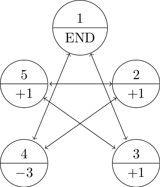
5. The transition probabilities are all equal to \(\frac{1}{2}\) and the transitions are dictated by the state diagram below.

Simulating Markov Pinball

There are a lot of ways to program this. We are going to show one way to do this and we invite our readers to find more efficient methods. In fact, the code that we are going to show, is purposefully not the most generic code that could be written.

One way to motivate and encourage students is to challenge them to find improvements. In this case, if students are told that there are better ways to program this simulation, my experience has been that they will find those better ways! Eventually, they can be asked a more open-ended question like, “Is there a better way to do this?” For the student new to the topic, something leading like, “There are better ways to do this, can you think of any improvements?” is a good ice-breaker.

As should always be the case, before we sit down and hack out some code, we should first map out what it is we want to do. We need to decide on two big things first:

1. How do we want to handle the transitions from one state to the next?
2. What types of statistics do we want to track?

The answer to both of these questions is dependent on the programmer. So there is not one correct answer. For me, because of instructional constraints, I have chosen to write this in a more static way. The statistics I want to keep track of are things like “total points accumulated”, “total points accumulated per state”, and “games played”.

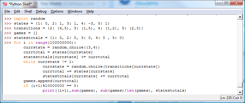
As such, I decided to go with this:

Now, this code I have left uncommented. I leave it as an exercise for the reader to determine if this adequately plays out 100 million games of Markov Pinball.

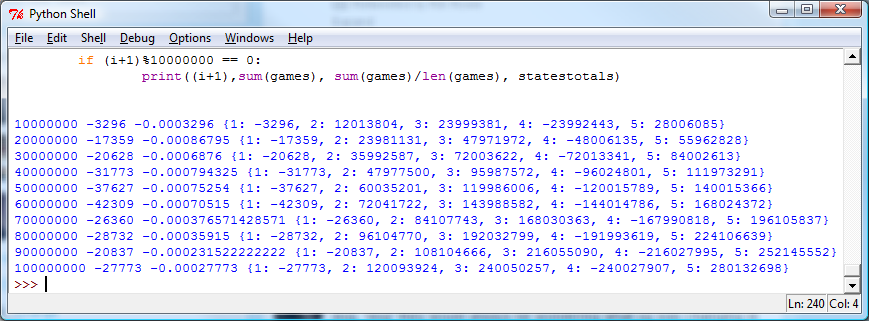
As for the output, I kept a running tally and printed the results every 10 million plays. Here are observed results along with the print statement from above:

What do we notice with these results?

• The total points accumulated after 100 million games was -27773, which translates to -0.00027773 points per game. Our theoretical calculations stated that we should have a net of zero. So how do we explain the negative results?
• How do the per state averages compare to our theoretical calculations?
• \(T_{3}\) and \(T_{4}\) were, in theory, supposed to be equal in magnitude. After 100 million plays, we do not have equality, but the numbers look close. How convinced are we that both our theory and computation are correct?

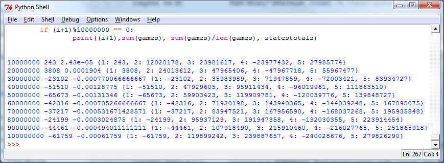
What happens if we reset our counters and ran another trial of 100 million game plays?

At 20 million plays, we were showing a slight positive return per game. At 30 million plays, our per game point accumulation was negative and stayed negative, but still stayed “close” to zero. Are we sure we got things right?

Check back on Monday as we start exploring some concepts from statistics. In the meanwhile, comment the code, think of other ways the code could have been written (say to keep things more generic), and think about what’s going on with these numbers.

Don’t hesitate to get in touch if you have questions or would like more information about setting up a workshop or training in your school.