Whether you’re teaching AP Stats or an introductory or senior level probability course for undergrads, you’ll know that students have a difficult time getting their minds wrapped around arithmetic for probability distributions. Here’s a simple example from the world of continuous probability.
Let \(X, Y\) be iid normal with mean zero and variance 1. Now we’ll have a question like
What is the distribution of \(Z = X – Y\)?
Now a typical course will have students go through the math symbolism mechanics to eventually arrive at \(Z \sim N(0,\sqrt{2})\), using the notation \(N(\mu,\sigma)\) rather than \(\sigma^{2}\). This is all good and well. But there’s often no visual follow up. Or even a sampling follow up.
Do me one favor, ask your students this simple but evil question.
Prove or disprove. Let \(X, Y\) be iid normal with mean zero and variance 1. If \(Z_{1} = X – Y\), \(Z_{2} = Y – X\), and \(Z_{3} = X + Y\) then \(Z_{1}\), \(Z_{2}\), and \(Z_{3}\) all follow the same distribution.
I like this question for a lot of reasons. Here are a few main reasons (and there are lots of smaller reasons, too many to enumerate).
- Coursework in a probability course is often focused on transformations of distributions while the comparison of one distribution to another is held off for a statistics course. I see the wisdom in the separation, but that doesn’t mean we can’t start preparing students for what’s to come.
- This question can be a headscratcher because sometimes students want to believe that if “\(X\) and \(Y\) are the same thing” (that’s the mistake), then their difference should be zero. Ah, but \(X\) and \(Y\) are not the same thing. They just have the same distribution but come from two independent, though identically distributed “streams”. I say “streams” because what’s lost in a probability course is the sampling aspect of all these distributions — the thing left for a stats course. We are drawing from \(X\) and drawing from \(Y\). So the first draw from \(X\) and from \(Y\) don’t produce identical values. The \(X – Y\) part of the question helps students to see the difference between that and \(X – X\) or \(Y – Y\).
- The second bullet point also helps separate the notion of “equality” when it comes to random numbers / processes. There’s equality in value and then there’s equality in distribution!
- Even if you don’t want to convert your probability course into a stats course, this is a great chance for visualizations!
- I will have a hard time believing that you won’t have a long discussion about this!
- Want a part deux? Compare \(\frac{X}{Y}\) against \(\frac{Y}{X}\).
Some Visualizations
Here are some visualizations. [Also, an end of the post plug: remember to subscribe!]
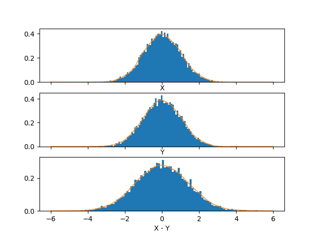
Ok, first it’s good to just take a look at what \(X\), \(Y\), and \(X-Y\) look like sampled (with a smoothed pdf overlaying them). (The histograms are normalized so they integrate to 1, rather than their height being their frequency.)
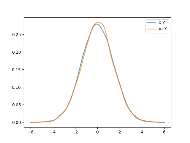
Next, here are fits for \(X-Y\) and \(X+Y\) based on 10,000 samples.
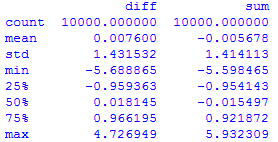
And finally, tables are visualizations too! (\(X-Y\)) is the “diff” column and (\(X + Y\)) is the “sum” column.